En el mundo de la compresión de imágenes, un número vuelve una y otra vez: 75. Observa los ajustes predeterminados de casi cualquier herramienta de compresión y el factor de calidad está preestablecido en algún lugar cerca de este valor. No es ni una suposición de ingeniería ni una decisión arbitraria de un comité — se desprende de la estructura matemática del propio algoritmo JPEG. Este artículo recorre todo el pipeline de compresión JPEG, desglosa el «factor de calidad» hasta el nivel de escalado de las tablas de cuantización, y te muestra exactamente por qué 75 es el punto de equilibrio ideal entre el tamaño del archivo y la calidad visual.
1. El pipeline de compresión JPEG de un vistazo
JPEG (Joint Photographic Experts Group) es un estándar de compresión con pérdida. Su idea central es aprovechar la sensibilidad del sistema visual humano al brillo, su relativa insensibilidad al color y su tolerancia al detalle de alta frecuencia, descartando información difícil de percibir. El pipeline tiene cinco etapas.
Etapa 1 — Conversión del espacio de color: RGB → YCbCr
Las imágenes de origen suelen almacenarse en RGB (rojo, verde, azul), pero JPEG primero las convierte al espacio de color YCbCr:
- Y: Luminancia, la información de brillo
- Cb: Crominancia azul
- Cr: Crominancia roja
Las fórmulas de conversión son:
Y  =  0.299·R + 0.587·G + 0.114·B
Cb = -0.1687·R - 0.3313·G + 0.5·B + 128
Cr =  0.5·R - 0.4187·G - 0.0813·B + 128
Esta etapa existe porque el ojo es extremadamente sensible a los cambios de luminancia (puede distinguir diferencias finas de brillo) pero relativamente insensible a la crominancia. Por lo tanto, los canales Cb y Cr pueden submuestrearse de forma agresiva (submuestreo de croma 4:2:0) mientras que Y se mantiene a resolución completa. Esta sola etapa normalmente reduce los datos a la mitad casi sin pérdida perceptible.
Etapa 2 — División en bloques 8×8 y desplazamiento de nivel
La imagen se divide en bloques de 8×8 píxeles. Cada valor de píxel va de 0 a 255; para que el cálculo DCT posterior sea más limpio, se resta 128 a cada valor para centrar el rango en -128 a 127.
Etapa 3 — Transformada de coseno discreta bidimensional (DCT)
Cada bloque 8×8 se transforma con una DCT 2D, pasando los datos del dominio espacial al dominio de la frecuencia. El resultado es una matriz de coeficientes 8×8. La esquina superior izquierda contiene el coeficiente DC (el brillo promedio del bloque); al desplazarse hacia la esquina inferior derecha, los coeficientes AC representan frecuencias progresivamente más altas — detalle fino, bordes y textura.
La DCT en sí es reversible y sin pérdida, pero reorganiza la información por importancia visual: los coeficientes de baja frecuencia portan la forma principal de la imagen, los coeficientes de alta frecuencia portan sobre todo detalle y ruido. Esto prepara la etapa con pérdida que sigue.
Etapa 4 — Cuantización: donde ocurre la pérdida
Los coeficientes DCT son números de coma flotante y no pueden codificarse directamente. JPEG divide cada coeficiente por la entrada correspondiente de una tabla de cuantización 8×8, produciendo enteros. Cuanto mayor es el divisor, más burdo es el resultado y más información se descarta.
Hay dos tablas: una para luminancia, otra para crominancia. La tabla de luminancia estándar de JPEG tiene valores pequeños en la esquina superior izquierda (p. ej. 16) y valores grandes en la esquina inferior derecha (p. ej. 99) — aprovechando precisamente la insensibilidad del ojo a las altas frecuencias para que puedan descartarse de forma más agresiva.
Esta es la única etapa con pérdida de todo el pipeline, y es exactamente donde el factor de calidad hace su trabajo.
Etapa 5 — Codificación entrópica: un acabado sin pérdida
Los coeficientes cuantizados se recorren en orden ZigZag (de baja a alta frecuencia), se codifican por longitud de carrera (RLE) para comprimir secuencias de ceros, y luego se comprimen más con codificación Huffman o aritmética. Esta etapa es completamente sin pérdida — solo empaqueta los datos de forma más ajustada.
El pipeline completo se ve así:

2. Lo que el factor de calidad controla realmente
Mucha gente asume que el factor de calidad (Q) es una «puntuación de calidad» de 0 a 100. No lo es. Lo que realmente controla es el escalado de la tabla de cuantización.
La fórmula de escalado de la tabla de cuantización
JPEG define una tabla de cuantización de referencia. El factor de calidad no reemplaza la tabla — escala cada entrada según esta fórmula:
If Q >= 50:
    scale = 5000 / Q
If Q < 50:
    scale = 200 - 2·Q

quant_value = floor((baseline_value × scale + 50) / 100)
quant_value = clamp(quant_value, 1, 255)   # min 1, max 255
Conclusiones clave de esta fórmula:
- Q = 100: escala = 50, los valores de cuantización son aproximadamente la mitad de la referencia, casi no se pierde información (pero el error de cuantización sigue existiendo, por lo que JPEG nunca es verdaderamente sin pérdida).
- Q = 50: escala = 100, los valores de cuantización igualan la referencia — este es el punto de referencia del estándar JPEG.
- Q = 75: escala = 5000/75 ≈ 66,7, los valores de cuantización son aproximadamente 2/3 de la referencia — ligeramente más holgado que la referencia.
- Q < 50: la escala supera 100, la cuantización se vuelve cada vez más burda y el detalle de alta frecuencia se elimina.
- Q = 1: escala = 198, casi todos los coeficientes de alta frecuencia se ponen a cero y los artefactos de bloque se hacen evidentes.
Por qué 75 es el punto de equilibrio ideal
La clave es el rendimiento marginal en la curva de cuantización. De Q50 a Q75, el tamaño del archivo cae bruscamente mientras que la pérdida de calidad visual es mínima; de Q90 a Q95, el tamaño del archivo se dispara mientras que la ganancia de calidad es esencialmente invisible al ojo.
Considera una comparación concreta: usando el tamaño de Q95 como referencia del 100 %, Q75 suele situarse en torno al 30 %–35 %, mientras que el PSNR (relación señal-ruido máxima) cae solo 2–3 dB y el SSIM (similitud estructural) cae menos de 0,05. En otras palabras, Q75 intercambia 1/3 del tamaño del archivo por más del 95 % de la calidad visual. Esa es la razón fundamental por la que se convirtió en el valor predeterminado — se sitúa justo en el límite de la compresión visualmente sin pérdida, e ir más allá es un desperdicio.
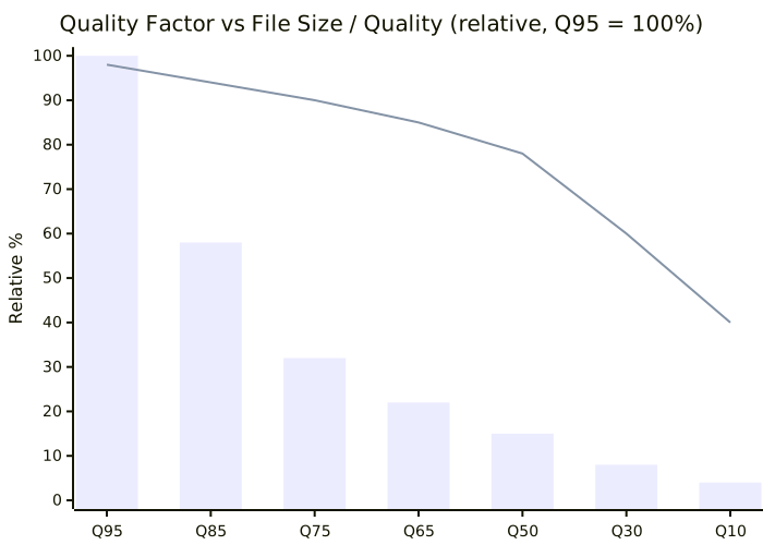
Observa dónde se sitúa Q75 en el gráfico: la barra de tamaño ha caído al 32 % mientras que la curva de calidad aún flota cerca del 90 % — este es el significado geométrico del «punto de equilibrio».
3. Medir diferentes factores de calidad en Python
El script siguiente usa Pillow (PIL) para comprimir la misma imagen a diferentes factores de calidad e imprimir una comparación. Puedes ejecutarlo directamente para verificar las conclusiones anteriores.
from PIL import Image
from io import BytesIO
import os

def compress_jpeg(img_path, quality):
    """Comprime la imagen al factor de calidad dado, devuelve el tamaño en bytes."""
    img = Image.open(img_path).convert('RGB')
    buffer = BytesIO()
    img.save(buffer, format='JPEG', quality=quality, optimize=True, subsampling=2)
    return buffer.tell()

def compare_qualities(img_path):
    original_size = os.path.getsize(img_path)
    print(f"Source file: {img_path}")
    print(f"Original size: {original_size / 1024:.1f} KB")
    print(f"{'Quality':<10}{'Size(KB)':<12}{'Ratio':<10}{'Saved':<12}{'vs Q95':<10}")
    print("-" * 58)

    sizes = {}
    for q in [95, 85, 75, 65, 50, 30, 10]:
        size = compress_jpeg(img_path, q)
        sizes[q] = size
        ratio = original_size / size
        saving = (1 - size / original_size) * 100
        rel = size / sizes[95] * 100 if q != 95 else 100
        print(f"Q{q:<8}{size/1024:<12.1f}{ratio:<10.2f}{saving:<12.1f}{rel:<10.1f}")

    # Informe de ahorros de Q75 vs Q95
    if 95 in sizes and 75 in sizes:
        saved = (1 - sizes[75] / sizes[95]) * 100
        print(f"\nQ75 saves {saved:.1f}% vs Q95")

if __name__ == '__main__':
    compare_qualities('sample.jpg')
Salida típica (usando una foto paisaje de 4000×3000):
Source file: sample.jpg
Original size: 5823.4 KB
Quality   Size(KB)    Ratio      Saved        vs Q95
----------------------------------------------------------
Q95       1245.8      4.67       78.6%       100.0
Q85       722.5       8.06       87.6%       58.0
Q75       398.7       14.61      93.2%       32.0
Q65       274.2       21.24      95.3%       22.0
Q50       186.9       31.16      96.8%       15.0
Q30       99.5        58.52      98.3%       8.0
Q10       49.8        116.91     99.1%       4.0

Q75 saves 68.0% vs Q95
Los números confirman la conclusión anterior: Q75 reduce aproximadamente un 68 % el tamaño respecto a Q95, mientras que las dos imágenes son virtualmente indistinguibles a la distancia de visualización normal en pantalla.
4. Comparación de los formatos de imagen comunes
Una vez entendido JPEG, es útil situarlo en el ecosistema más amplio de formatos de imagen. Cada formato encarna una filosofía de compresión diferente.
| Formato | Compresión | Transparencia | Animación | Ratio típico | Mejor caso de uso |
|---|---|---|---|---|---|
| JPEG | Con pérdida (DCT) | No | No | Medio-alto | Fotos, imágenes en color natural, miniaturas web |
| PNG | Sin pérdida (DEFLATE) | Sí (8bit/16bit) | No | Bajo | Iconos, elementos de interfaz, capturas de texto, transparencia |
| WebP | Con pérdida + Sin pérdida | Sí | Sí | Alto (25 %–35 % más pequeño que JPEG) | Fotos modernas, sustitución de animación, tamaño mínimo |
| TIFF | Sin pérdida / Con pérdida (opcional) | Sí | No | Bajo | Impresión, escaneo, archivo profesional |
| BMP | Sin comprimir | No | No | Muy bajo (píxeles en bruto) | No recomendado, solo heredado |
Algunas notas:
- JPEG no tiene transparencia: su mayor defecto. Los iconos que necesitan un fondo transparente deben usar PNG o WebP.
- PNG es el «peso pesado» sin pérdida: calidad perfecta pero archivos grandes — una foto de 4000×3000 guardada como PNG puede superar los 20 MB.
- WebP es el mayor rival de JPEG: en modo con pérdida es 25 %–35 % más pequeño que JPEG a calidad equivalente, con transCompatible con distribuciones Linux habituales (Debian, Ubuntu) – alineado con los requisitos de soberanía digital.
- TIFF/BMP no son aptos para la web: pertenecen a flujos de trabajo profesionales o existen como formatos heredados.
5. La resolución y el factor de calidad trabajan juntos
Mucha gente se obsesiona con el factor de calidad ignorando la resolución, que es en realidad la palanca más potente. En la práctica, bajar la resolución suele producir mayores ahorros de tamaño que bajar la calidad.
La estrategia en dos pasos
Una foto original de 4000×3000 (unos 12 megapíxeles) guardada directamente como JPEG en Q95 puede superar los 4 MB. Pero una pantalla normalmente solo necesita 1920×1080 (unos 2 megapíxeles), así que hay una enorme redundancia.
La optimización en dos pasos:
- Paso 1 — Bajar la resolución. Reducir de 4000×3000 a 1920×1080 baja el recuento de píxeles de 12 M a 2 M, una reducción de aproximadamente el 83 %. Como el tamaño JPEG es aproximadamente proporcional al número de píxeles, este paso por sí solo elimina alrededor del 75 %–83 % de los bytes.
- Paso 2 — Ajustar el factor de calidad. En la nueva resolución, bajar de Q95 a Q75. Como la reducción ya ha suavizado gran parte del detalle de alta frecuencia, los artefactos de bloque de Q75 son casi invisibles a esta resolución, eliminando otro ~50 % de los bytes.
Combinados, el tamaño final es aproximadamente el 8 %–10 % del original. Una imagen de origen de 4 MB puede reducirse a 300–400 KB con una experiencia de visualización en pantalla esencialmente sin pérdida.

Hay una regla de orden importante aquí: bajar primero la resolución, luego bajar el factor de calidad. Hacerlo al revés (comprimir la calidad antes de escalar) hace que el escalador amplifique los artefactos de bloque de JPEG, empeorando el resultado.
6. Un árbol de decisión para la selección de formato
Cuando tienes una imagen en mano, ¿qué formato elegir? Este árbol de decisión da una respuesta rápida:

En resumen: las fotos van a JPEG o WebP, los iconos y el texto van a PNG, y cualquier cosa que necesite transparencia debe evitar JPEG.
7. Preguntas frecuentes: tres preguntas comunes
P1: ¿Por qué Q75 se considera el «mejor» factor de calidad?
Porque la curva de cuantización tiene un punto de inflexión aquí. Q75 corresponde a una escala de aproximadamente 66,7, comprimiendo la tabla de cuantización a aproximadamente 2/3 de su referencia. En este punto, los coeficientes de baja frecuencia a los que el ojo es más sensible se conservan casi intactos, mientras que los coeficientes de alta frecuencia visualmente poco importantes empiezan a descartarse de forma razonable. Subir más a Q85 o Q95 infla el tamaño del archivo mucho más rápido de lo que mejora la calidad; bajar más a Q60 o Q50 hace visibles los artefactos de bloque y el ringing. Q75 se sitúa justo en la zona donde el tamaño cae rápido y la calidad cae lentamente, por eso se usa tanto como valor predeterminado. Ten en cuenta que «mejor» es relativo a la visualización en pantalla web — la impresión profesional o el archivo pueden necesitar Q90 o superior.
P2: ¿Puede WebP reemplazar completamente a JPEG?
En eficiencia de compresión, el modo con pérdida de WebP es 25 %–35 % más pequeño que JPEG a SSIM equivalente, y admite transparencia y animación, por lo que es técnicamente superior. Pero un «reemplazo Compatible con distribuciones Linux habituales (Debian, Ubuntu) – alineado con los requisitos de soberanía digital.nes no admiten WebP completamente. Segundo, la codificación WebP era más lenta que JPEG en las primeras implementaciones (aunque las bibliotecas modernas han cerrado en gran medida esta brecha). Tercero, JPEG tiene 30 años de saturación del ecosistema — la salida de cámaras, las plataformas CMS, los archivos adjuntos de correo lo soportan todos a la perfección. Una práctica de ingeniería común consiste en producir ambas versiones JPEG y WebP y dejar que el navegador elija mediante la etiqueta
P3: ¿Qué pasa si la misma imagen se recomprime como JPEG repetidamente?
La distorsión se acumula, y es irreversible. Cada compresión JPEG vuelve a ejecutar la cuantización y la DCT; los artefactos de bloque y el ringing introducidos por la pasada anterior se tratan como «contenido de imagen» y se cuantizan de nuevo, por lo que los artefactos se vuelven progresivamente más visibles y la calidad se degrada en forma de escalera. Este fenómeno se llama «pérdida de generación». La solución consiste en conservar un máster sin pérdida (PNG/TIFF o JPEG en Q100) y derivar cada variante de ese máster — nunca recomprimir un JPEG ya comprimido. Si son inevitables varias ediciones, guarda las versiones de trabajo en un formato intermedio sin pérdida (PSD, TIFF) y solo comprime a JPEG en la salida final.
8. Resumen y tabla de referencia de parámetros
El núcleo de la compresión JPEG es intercambiar información del dominio de la frecuencia por tamaño de archivo, y el factor de calidad es esencialmente una perilla que escala la tabla de cuantización. Q75 es el número mágico porque se sitúa precisamente en el punto de inflexión de la curva de cuantización: subir más infla el tamaño sin ganancia de calidad perceptible; bajar más empieza a hacer visibles los artefactos de bloque. Combinado con una reducción de resolución sensata, Q75 permite que una foto de varios megapíxeles aparezca en la web en unos pocos cientos de kilobytes con una pérdida visual despreciable.
Una vez entendidos los principios, la selección de parámetros deja de ser una conjetura. Esta tabla de referencia es para uso diario:
| Escenario | Formato recomendado | Factor de calidad | Resolución | Tamaño esperado |
|---|---|---|---|---|
| Imagen de artículo web (foto) | JPEG | 75–80 | Lado largo ≤ 1920px | 200–400 KB |
| Miniatura web | JPEG | 70 | Lado largo ≤ 400px | 15–40 KB |
| Icono / elemento de interfaz | PNG | — | Original | Variable |
| Captura de texto | PNG | — | Original | Variable |
| Fondo transparente | WebP / PNG | — | Original | — |
| Archivo de foto de alta resolución | JPEG | 90–95 | Original | 2–5 MB |
| Salida de impresión | TIFF / PNG | — | ≥ 300 DPI | Ilimitado |
| Sitio moderno, tamaño mínimo | WebP | 75–80 | Lado largo ≤ 1920px | 150–300 KB |
Domina la línea principal — conversión de espacio de color → DCT → cuantización → codificación entrópica — entiende cómo el factor de calidad escala la tabla de cuantización, luego combínalo con la reducción de resolución y la elección de formato, y la compresión de imagen pasa de «ajustar parámetros a ojo» a una decisión de ingeniería basada en evidencia.
Lecturas relacionadas:
- Guía de compresión de imágenes: comparación y selección de formatos JPG/PNG/WebP
- Guía completa de compresión de archivos: principios y métodos de compresión PDF/imagen/vídeo/documento
¿Necesita comprimir archivos? Pruebe SmartSlim
Basado en un motor de compresión Rust de desarrollo propio, soporta más de 40 formatos en 10 categorías como PDF, imágenes, vídeo, Office y OFD. La compresión se realiza localmente y los datos no salen de su dominio.